Quarto

Professional Writing in Political Science

Before I even start this section, please read Professional Writing in Political Science: A Highly opinionated Essay by James A. Stimson. The article is opinionated, but there is plenty of excellent advice in it on how to approach writing a research project. And that is, after all, what we learn quantitative methods for.

Introduction to Quarto

Stimson rejects Word and other similarly inclined word processing programs, as they are unable to achieve the standard required in professional academic writing. In the context of tables, for example, Stimson writes

You are a professional author. Learn to use the tools of authorship or choose a profession for which you are better suited.

I agree. And I wish more people, students and faculty members alike, would take note of this. The good news for you is that R, amongst the many other millions of things that this program enables us to do, provides an interface to write with Quarto.

Writing a quantitative research project in Quarto has some very notable benefits, such as great formatting, the seamless integration of graphs and results tables, and a semi-automatic list of references.

But what is Quarto? Quarto is “an open-source scientific and technical publishing system”¹. When we use it in R, the document will have essentially three parts:

• YAML
• Text
• Code Chunks

I will go through these in turn now. To follow along, I recommend you download the Assessment Template I wrote for my Determinants of Democracy module, PO33Q. Once you open it, delete the hashtag in the first line, so that Line 1 only contains three dashes ---. Otherwise, don’t do anything with it, yet. But whilst you are reading what I am discussing here, try to match it to what you see in the qmd file. If you want to jump ahead and render it into a pdf, please follow the instructions in the template section.

Once you open the essay template in R Studio, you will obtain a few more options in the task bar at the top which will allow you to turn this raw file into a pdf. More on this below, under “Rendering”.

It is possible that R will ask you to install the quarto package. Please do so, and also allow the installation of any dependencies if prompted.

YAML

YAML is an acronym for “Yet Another Markup Language”. This section of the document usually contains the settings for the entire document, such as the title, information about the bibliography (see below), and additional packages we might need to load. The YAML is gated by three horizontal dashes at the top and at the bottom. In the template, there is some more formatting going on outside of the YAML and finishes at line 136.

Text

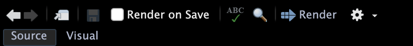
Then, in line 139, follows the text which you can basically type as you always would. In order to use the familiar text formatting icons that turn text into headings, or into bold, change the font size, etc. you can switch the Quarto editor to “Visual” at the top. In the template, this is set to “Source” where Quarto would expect code to achieve all of these formatting operations.

Once you activate it, this task bar will appear at the top of the qmd file:

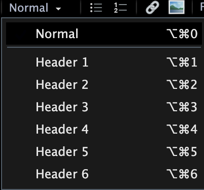
When you structure your document, it is essential that you format headings as such in the document and don’t just make the font larger. Otherwise, the automated table of contents will not work.

The visual editing bar will also allow you to include external pictures (external in the sense that you are not creating them in R whilst creating the document). For this purpose, click on the image icon in the visual editing bar, and a new window will pop up. Under the tab “Image” you can select the image from a file in your computer. Be sure to add a caption in this tab, as well. This will be printed underneath the image in your pdf. Then click the tab “Attributes”, and in the box “ID” enter a unique identifier for the image you are inserting. I usually use “fig” for figure, a colon, and then the name of the figure:

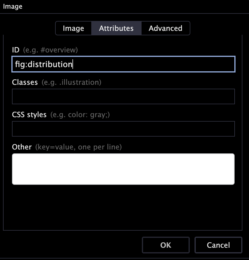
Once you have done that, click OK, and the image will appear where you have placed it. Because you created a caption and a label, you can now refer to this picture in the text, using the \ref{} function. When you write

As we can see in Figure \ref{fig:distribution} ...,

R will insert a cross reference which will get updated automatically when you render the document. This has the advantage that you will never have to say “the figure below” or the “figure above”. This is both imprecise and dangerous, as the position of the figure might change as you write your assessment.

You can also set beautiful equations in quarto Unless you really want to explain what conditional probabilities are in the the methods section of your assessment, I don’t think you will have to use this feature, however.

Code Chunks

As I mentioned in the introduction, one of the perks of writing an assignment in Quarto is that you can automate the generation of results tables. You can hide all of the ugly code, and just show a beautifully formatted table at the end. How do you do that? There are quite a few packages around to do this, but the best and most adaptable to my mind is modelsummary. To get started, please switch from the “Visual” mode back to “Source”. You can return to “Visual” editing mode once you are done with this.

To include raw R code in a Quato dicument, we need to create a code chunk, such as this:

```{r}
#| echo: false
#| message: false
#| warning: false

library(tidyverse)
```

To produce such a fence, there is a shortcut available on Mac and Microsoft:

• Mac: Option + Command + i
• Windows: Ctrl + Alt + i

In the chunk above, I have set the option echo: false which prevents the raw R code being shown in the rendered document. I have done the same thing for warnings, and messages. This should cover you for the creation of results tables.

To start, we need to load two packages, modelsummary and tinytable. We will use tinytable to adjust the style of the “default” table produced by modelsummary.

library(modelsummary)
library(tinytable)

Let us now run three regression models with some data taken from the carData package, so we have something to display in our table:

library(carData) # only needed for data to illustrate this here

data("Prestige", package = "carData") # only needed for data to illustrate this here

m1 <- lm(prestige ~ education, data = Prestige)
m2 <- lm(prestige ~ income + type, data = Prestige)
m3 <- lm(prestige ~ education + income, data = Prestige)

To produce the table, our first step is to store the results of all three regression models in a list:

models <- list("(1)" = m1, "(2)" = m2, "(3)" = m3)

By default, the results table would print the variable names in the left hand side column (called the stub). But this is not good practice, as variable names are often cryptic and won’t allow a reader to understand the results without looking at the table (something Stimson is very adamant about). So let’s replace the variable names with their labels in a so-called coefficient map. The order in which you place the variables in this map will be replicated in the results table:

cm <- c(
  "education"   = "Years of Education",
  "income"      = "Average Income",
  "(Intercept)" = "Constant"
)

Finally, the table itself. There is a lot going on in the following code chunk, and so I have annotated it, rather than delivering an endless explanation here in the text.

# Create the modelsummary table
modelsummary(models, 
             title = "Regression Models",     # this is the caption/title of the table
             gof_omit = 'DF|Deviance|Log.Lik|F|AIC|BIC|RMSE', # control goodness of fit measures
             stars=TRUE,                                    # info on statistical significance
             coef_map = cm,                                 # the coefficient map
             escape = FALSE,                                # needed for spacer below
             notes = "\\vspace{0.1\\baselineskip}",         # add space before caption
             notes_append = TRUE)|>                         # this is the custom row
  group_tt(j = list("Bivariate" = 2:3, "Multivariate" = 4)) |> # emergence/survival in assignment
  group_tt(j = list("Dependent Variable: Prestige Score" = 2:4))|> # add header
  theme_latex(outer = "label={tblr:regmodels}")|>           # label for crossref
  theme_latex(placement= "H")|>                             # place table [H]ere
  theme_latex(resize_width= 0.5, resize_direction="both")   # adjust table size (% of textwidth)

Regression Models

	Dependent Variable: Prestige Score
	Bivariate		Multivariate
	(1)	(2)	(3)
+ p < 0.1, * p < 0.1, ** p < 0.05, *** p < 0.01
Years of Education	5.361***		4.137***
	(0.332)		(0.349)
Average Income		0.001***	0.001***
		(0.000)	(0.000)
Constant	-10.732**	27.997***	-6.848*
	(3.677)	(1.801)	(3.219)

Because we have included a label, you can now refer to this table with a cross-reference in the text, for example by writing As we can see in Table \ref{tblr:regmodels} .... For more information on styling options, please consult the modelsummary webpage. I have split the code chunks into smaller parts for explanatory purposes here, but you can do all of this in one, big code chunk, such as this:

```{r, echo=FALSE, message=FALSE, warning=FALSE, error=FALSE}
# set your wd
setwd()

# load packages
library(modelsummary)
library(tinytable)

# load data

# carry out the analysis

# write the modelsummary code
modelsummary()

```

It is important that none of the code in this mini-script produces any visible output (everything needs to be carried out quietly and would not produce output in the console if executed from an R Script), as these results will otherwise appear in the final document. It almost goes without saying that the data set you are analysing will also have to be present in the folder that contains the qmd file².

I recommend you use a regular RScript to carry out the analysis, as you can execute commands, and play around with this more easily (rather than rendering the entire thing every time). Once you are happy with the output, create the chunk in the .qmd file and copy/paste your code.

List of References

OK, the biggest selling point of this is probably that Quarto will auto-generate a complete list of references by pressing a button. By the way, do you know what the difference is between a bibliography and a list of references?

A bibliography lists all sources you have consulted for a project regardless of whether they are cited in the text, whereas a list of references only lists what has been cited in the text.

Warning:

The PAIS UG Handbook wants you to produce a list of references, but calls it a bibliography 🙄. Please produce a list of references, and call it “List of References” in this assessment. You know better now.

This list of references must:

• be organised alphabetically by surname of author
• not be in bullet points
• consistently formatted
• preferably APA styled, but I’m not too precious as long as it’s consistent

I wrote earlier that generating the list of references is semi-automatic, because – as you will have come to realise by now – there is no such thing as a free lunch. The process requires a little preparation, and I am afraid some in-text code.

First, you need to create a separate file in which all of the sources you wish to cite are hosted – a so called .bib file. You can download the full .bib file for each module I teach in the Downloads Section of my GitHub page, in the hope that it already covers some sources you may wish to cite in your assessment. You can open this file in R Studio. As you will see, the structure of each entry depends on the type of document you are citing: a book, an article in a journal, or a website, for example. Here is an entry for a book:

@Book{prz:2000,
  author    = {Adam Przeworski and Michael E. Alvarez and Jos\'e A. Cheibub and Fernando Limongi},
  publisher = {Cambridge: Cambridge University Press},
  title     = {{Democracy and Development - Political Institutions and Well-Being in the World, 1950-1990}},
  year      = {2000},
  doi       = {10.1017/CBO9780511804946},
}

In this entry, prz:2000 is called the citation key. This is what you will use in the qmd file. For example when you type \citep{prz:2000} this will be shown as (prz:2000?) in the final document. In the template, I have enabled the following styles for including a reference in the text:

Input	Output
\citep{prz:2000}	(Przeworski et al., 2000)
\citep[p. 20]{prz:2000}	(Przeworski et al., 2000, p. 20)
\citep[see][p. 20]{prz:2000}	(see Przeworski et al., 2000, p. 20)
\citet{prz:2000}	Przeworski et al. (2000)
\citet[p. 20]{prz:2000}	Przeworski et al. (2000, p. 20)
\citet[see][p. 20]{prz:2000}	see Przeworski et al. (2000, p. 20)

When you render the essay template, Quarto will automatically put a list of references together and place it where it belongs³. But how do you render the document?

Rendering

To convert the qmd file to a pdf, you will have to “render” the qmd file. An icon with an arrow is located in the task bar at the top whenever you have an qmd file open. Click it to start the conversion.

When there is a mistake in your qmd file, such as an unbalanced bracket in a code chunk, for example, R will not render the pdf. Therefore, knit your document regularly, so that you can trace the error more easily.

Assessment Template

In order to make your life as easy as possible, I have put together an Assessment Template in the form of an qmd file that you can knit in R. The template is for for my Determinants of Democracy module (PO33Q), but you can easily adapt it to suit the needs for assessments on other modules. You can download it here. In order to knit this document, you need to remove the hashtag in the first line, so that line 1 only contains three dashes ---, and place the following files in the same folder as the qmd file:

• Warwick Crest for the title page.
• Warwick Text for the title page.
• referencesPO33Q.bib which contains all entries for the complete bibliography of the module.

Render / knit this document without making any changes to ensure this works. It should look like this. Then you can start writing your assessment. Again, let me encourage you to render/knit the document often, so that you can locate a potential mistake more easily should you receive an error message.

The Template Explained

There is quite a bit of formatting going on in the qmd file, and this is what all of this code achieves:

• Light grey background to improve readability (a little present to myself for marking)
• Font size 12, one-half spacing
• Main font: Latin Modern Sans Serif for legibility
• Maths font: Fira Maths, ditto
• Title page with module name, your registration number, submission date, and word count. No page number.
• Page numbering in Roman numerals for table of contents, list of figures, and list of tables
• Table of contents, list of figures, and list of tables are automatic
• Page numbering in Arabic numerals from the start of the text
• All captions are placed beneath figures and tables
• Fully adjustable size of modelsummary table (controlled via percentage of text width), so you can control the number of words the table “costs”
• Automatic page break if there are fewer than seven lines after a (sub-)section heading
• Automatic List of References, formatted in APA (American Psychological Association) style
• Appendix after the List of References
• Code chunks are set by default not to show the code in the rendered file. Messages, warnings, and errors are suppressed

Assessment Submission

When it comes to submitting your assessment, please only submit the rendered pdf, and NOT the qmd file. This will not be accepted by Tabula. If you wish to use Quarto on modules other than those taught by me, then please consult the module director whether they are happy to accept submissions in pdf format.

For the purpose of reproducibility, please ensure that you have copied and pasted your complete RScript into the Appendix section of the template. By complete I mean a script that takes you (or anybody else) from loading the original data set (“as is”) to the output you include in the assignment you submit on Tabula. The script should be properly annotated to make your work reproducible and easy to follow.

---

1. https://quarto.org/

2. You can create absolute and relative file paths to other locations, but let’s not over-complicate things here.

3. Otherwise, this will be placed into the document as the very last thing, but because you have an appendix, I needed to overrule this behaviour in the template.